ML On Edge : Create, Deploy and Infer

Ever since Machine learning term introduced by Prof. Arthur Samuel (Stanford University) in 1959 , Machine learning is a famous word in tech industry. However back propagation techniques and GPUs made it to next level in last decade, Recent advancement is running ML on edge using Tflite.
In this blog, we shall do the model preparation, model conversion at companion desktop /server, model deployment and inference on edge.

• Model Preparation
• Model conversion
• Model deployment and debugging
• Running inference

Instead of writing everything in one blog, I am gonna break it into two different blogs, I will discuss the first two topics in this blogs and remaining in the later blogs

Model Preparation

What is machine learning Model ?

In a typical programming world, when an input is given, it will undergo some processes or trigger new processes to get desired output. While machine learning makes use of inputs and makes predictions or classifications on the unknown data (or data near to that of training data). To do this task of prediction or classification, we need to make use of training and create model. For simplicity, I am considering prediction model here. By using known data set and its behavior, create a pattern in a way that when a new data is provided, this pattern will be able to tell (predict) the output.

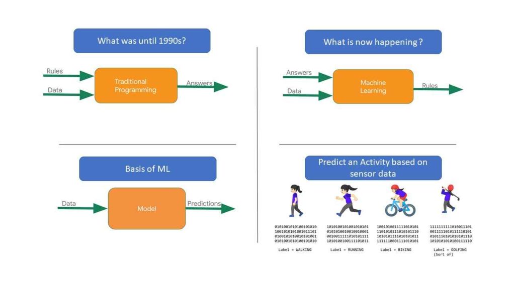
Data set is collection of entries where we know the mapping between input and output. (there are other kinds of data sets where we only have inputs, on which we can use unsupervised learning algorithms). Generally for a machine learning problem, the data set is divided into 3 sets

• Training data set
• Testing data set
• Validation data set

Training dataset has to be applied on the model
Once we’ve defined the model, we can use our data to train it. Training involves passing an x value into the neural network, checking how far the network’s output deviates from the expected y value, and adjusting the neurons’ weights and biases so that the output is more likely to be correct the next time.
Let us understand what model is with an example.
Consider the parameters below ( given x and corresponding y)

x =  [-10,-9,-8,-7,-6,-5,-4,-3,-2,-1,0,1,2,3,4,5,6,7,8,9,10,11] 
y =  [-23.33,-22.78,-22.22,-21.67,-21.11,-20.56,-20.00,-19.44,-18.89,-18.33,-17.78,-17.22,-16.67,-16.11,-15.56,-15.00,-14.44,-13.89,-13.33,-12.78,-12.22,-11.67] 

There is some relationship between these two values , based on that relationship how to predict the value of Y when new x value is given is the problem. Y is function of x

In Machine learning, this phenomenon of finding the corresponding relationship between X & Y is called model. This can be simple straight line ,or quadratic two degree curve or polynomial curve

When the computer is trying to ‘learn’ that, it makes series of guesses…to start with `y=23x+32`. The `loss` function measures the guessed answers against the known correct answers and measures how well or how badly it did.
Next, the model tries to optimize the function (this term is optimizer parameter in NN). Based on the previous loss function’s result, it will try to reduce the loss. At this point maybe it will come up with something like `y=(x-32)*0.9`. While this is not yet correct function, nevertheless it’s closer to the correct result (whereby. the loss is getting minimum and minimum).
The model will repeat this for the number of times (this term is known as epochs in NN)
This oss can be calculated by`mean squared error` for the loss (squaring is done to nullify positive and negative values) and `stochastic gradient descent` (sgd) for the optimizer. Let us not bother about what these terms for now, They are my optimizer functions. Later we will learn the different and appropriate loss and optimizer functions for different scenarios.

Let us use Jupyter notebook to try these and create our first model

#Step 1 Import statements to get all the necessary packages
import tensorflow as tf
import numpy as np
from tensorflow import keras
#step 2 define model, with single value, single layer
model = tf.keras.Sequential([keras.layers.Dense(units=1, input_shape=[1])])
model.compile(optimizer='sgd', loss='mean_squared_error')
#step 3 define the X and y values for which we need to find function 
xs = np.array([-10,-9,-8,-7,-6,-5,-4,-3,-2,-1,0,1,2,3,4,5,6,7,8,9,10,11], dtype=float)
ys = np.array([-23.33,-22.78,-22.22,-21.67,-21.11,-20.56,-20.00,-19.44,-18.89,-18.33,-17.78,-17.22,-16.67,-16.11,-15.56,-15.00,-14.44,-13.89,-13.33,-12.78,-12.22,-11.67], dtype=float)
#step 4 let us train our model on this values by fitting them
model.fit(xs, ys, epochs=500)
#step 5 get new value of Y for given X
print(model.predict([42]))

Little observation will tell us that these are Celsius and Fahrenheit Y= (X-32)*5/9
Model says 5.555244 where as actual answer is 5.56

Having understood what model is, let us make up another model to deploy on edge.
To make it simple , consider the Cosine model (typically all learning material takes up sine model including google codelab, to be different, Let us take up Cosine)

#Make bigger sample data set of 1000
SAMPLES = 1000
#seed value ensures same randomness occurs everytime we run the program
np.random.seed(1337)
#Generate a uniformly distributed set of random numbers in the range from
#-pi/2 to 3π/2, which covers a complete cosine wave oscillation
x_values = np.random.uniform(low=-math.pi/2, high=3*math.pi/2, size=SAMPLES)
#Shuffle the values to guarantee they're not in order
np.random.shuffle(x_values)
#Calculate the corresponding cosine values
y_values = np.cos(x_values)
#Plot our data. The 'b.' argument tells the library to print blue dots.
plt.plot(x_values, y_values, 'b.')
plt.show()

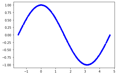
This is smooth function (no noise in the data). Let us add some noise to the data by tweaking the data a bit.
Thus we will get variation in the data and then we shall find relationship

y_values -= 0.1 * np.random.randn(*y_values.shape)
plt.plot(x_values, y_values, 'b.')
plt.show()

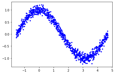
Now the relationship is not smooth and points got scattered. Let us find the model using tensorflow for these points

#65 and 20 will be used for training, testing, remaining 15 % will be used for validation
TRAIN_SPLIT =  int(0.6 * SAMPLES)
TEST_SPLIT = int(0.2 * SAMPLES + TRAIN_SPLIT)
x_train, x_test, x_validate = np.split(x_values, [TRAIN_SPLIT, TEST_SPLIT])
y_train, y_test, y_validate = np.split(y_values, [TRAIN_SPLIT, TEST_SPLIT])
#confirm that our splits add up correctly to 100
assert (x_train.size + x_validate.size + x_test.size) ==  SAMPLES
#Plot the data in each partition in different colors:
plt.plot(x_train, y_train, 'g.', label="Train")
plt.plot(x_test, y_test, 'r.', label="Test")
plt.plot(x_validate, y_validate, 'b.', label="Validate")
plt.legend()
plt.show()

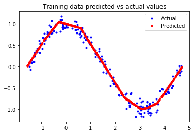
The result function is more or less coincide with actual cosine function,.however there few straight line area. Let us refine it

model_2 = tf.keras.Sequential()
#First layer takes a scalar input and feeds it through 16 "neurons". The
#neurons decide whether to activate based on the 'relu' activation
function.model_2.add(layers.Dense(16, activation='relu', input_shape=(1,)))
#The new second layer may help the network learn more complex representations
model_2.add(layers.Dense(16, activation='relu'))
#Final layer is a single neuron, since we want to output a single value
model_2.add(layers.Dense(1))
#Compile the model using a standard optimizer and loss function for regression
model_2.compile(optimizer='rmsprop', loss='mse', metrics=['mae'])
#Make predictions based on our test dataset
predictions = model_2.predict(x_test)
#Graph the predictions against the actual values
plt.clf()
plt.title('Comparison of predictions and actual values')
plt.plot(x_test, y_test, 'b.', label='Actual')
plt.plot(x_test, predictions, 'r.', label='Predicted')
plt.legend()
plt.show()

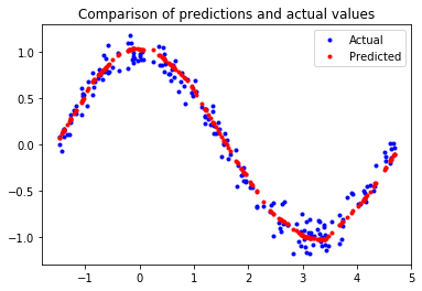
Now the model is closely looking like cosine curve
Model predicted by Tensorflow NN is more or less similar to Cosine Wave.

Now save this model and convert it to tensorflow lite to use it in the Edge

keras_file = "keras_model.h5"
tf.keras.models.save_model(model_2, keras_file)
converter = tf.lite.TFLiteConverter.from_keras_model_file("keras_model.h5")
tflite_model = converter.convert()
converter.optimizations = [tf.lite.Optimize.OPTIMIZE_FOR_SIZE]
open("cosine_qunantized_model.tflite", "wb").write(tflite_model)

Now use this tflite file to generate c data file (run the following in terminal)

 xxd -i sine_model_quantized.tflite > sine_model_quantized.cc

Include this model data and predict the values. In next blog we will see how to deploy and infer using this model.

In this blog, we understood what data model is?, how to generate it using TF, and convert into tflite to use it in edge

Share your views.